
Land ice
Conventionally, the mass balance of glaciers and ice caps (GIC) and the ice sheets, have been treated as separate problems, using different approaches and assumptions.
In-situ and geodetic measurements of GIC mass and volume changes extend back multiple decades with a handful of glacier length records going back to ~1860 [1] and various approaches have been used to upscale these to provide global estimates (e.g. [2]). By contrast, robust, observational estimates of ice sheet mass balance begin with the launch of ESA’s satellite, ERS-1, in 1991.
This partly explains the difference in approach used but there is also an issue of scale. The Antarctic ice sheet is larger than the conterminous United States and extrapolation of a small number of poorly distributed in-situ observations is not a viable approach.
Since the early 1990s, three approaches have been adopted for determining ice sheet mass balance: the Input- Output Method (IOM), elevation change (dh/dt) from satellite and airborne altimetry, and changes in the gravity field from GRACE. Each approach involves different errors in space and time, but also represents a different “type” of information about mass balance.
Therefore combining them into a joint inference is far more powerful and informative than considering them separately or taking, say, the arithmetic mean of multiple estimates. However, in this combined approach it is essential to understand how the different errors are correlated, across datasets and within datasets, across space and time. The image below shows an example of RATES results for Antarctica, where a static GIA field and time-evolving ice dynamics and surface process fields were solved simultaneously (e.g. [3]).
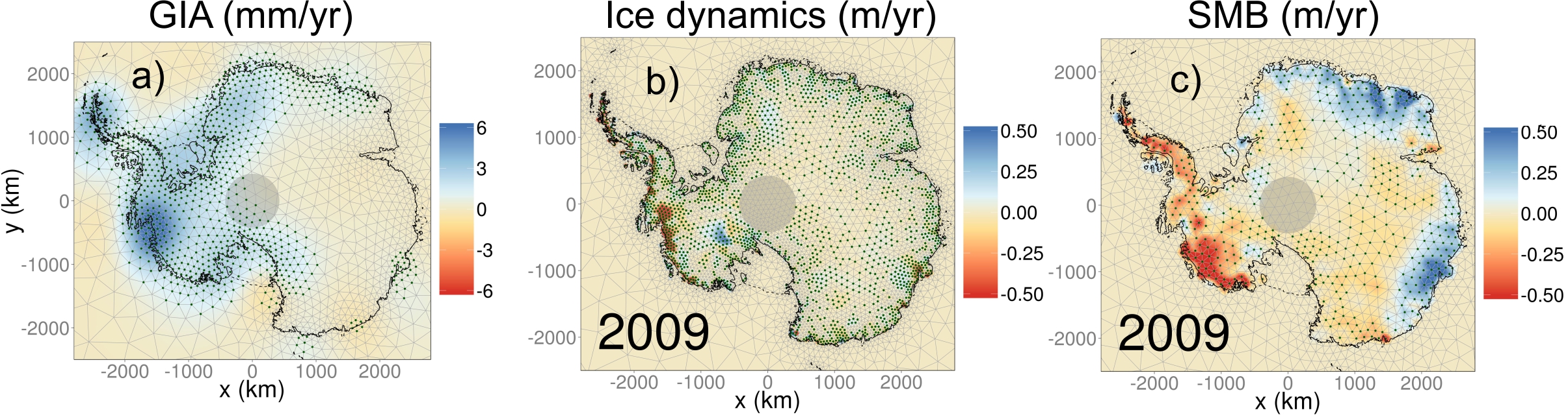
The BHM solution (posterior mean) from the RATES project for a) GIA vertical bedrock velocity, b) ice surface elevation change (dh/dt) due to ice dynamics for 2006 and c) dh/dt due to anomalies in surface mass balance (predominantly snowfall) in Antarctica in 2006. GIA is time invariant. The green hatching indicates where the amplitude of the signal is statistically significant. The standard error is also produced at the same resolution for each year (not shown).
This demonstrates a number of important points about our approach. The spatial resolution for each process (defined by the triangular meshes) does not have to be identical between, or within, a process. Where gradients are large, resolution can be high and vice versa. This is important for computational efficiency and is possible because of the use of stochastic partial differential equations (SPDEs) for the process model in the BHM.
Next page: Progress
References
[1] Vaughan, D. G., J. C. Comiso, I. Allison, J. Carrasco, G. Kaser, R. Kwok, P. Mote, T. Murray, F. Paul, J. Ren, E. Rignot, O. Solomina, K. Steffen and T. Zhang (2013). Observations: Cryosphere. Climate Change 2013: The Physical Science Basis. Contribution of Working Group I to the Fifth Assessment Report of the Intergovernmental Panel on Climate Change. T. F. Stocker, D. Qin, G.-K. Plattner et al. Cambridge, United Kingdom and New York, NY, USA, Cambridge University Press: 317–382.
[2] Marzeion, B., A. H. Jarosch and M. Hofer (2012). “Past and future sea-level change from the surface mass balance of glaciers.” The Cryosphere 6(6): 1295-1322.
[3] Zammit-Mangion, A., J. Rougier, N. Schön, F. Lindgren and J. Bamber (2015). “Multivariate spatio-temporal modelling for assessing Antarctica’s present-day contribution to sea-level rise.” Environmetrics 26(3): 159-177.