

With a full project team finally in place from late 2019, making progress on the key research aims and objectives was the main focus of our work during 2020 – something that was made somewhat more complicated by the coronavirus pandemic and subsequent need to work remotely from March 2020 onwards.
Despite this unforeseen challenge, work began in earnest to develop our Bayesian Hierarchical Model (BHM) to investigate GIA and mass trends for North America. We chose North America as it represents a ‘data rich’ region, allowing us to develop and test the BHM over a discrete area for a smaller number of relatively well observed (and understood) processes.
(1) GIA and mass trends for North America
Over North America, we were essentially only concerned with two processes – vertical land motion and hydrology – as observed by GPS stations and GRACE gravimetry. However, and as we came to learn, behind that seemingly simple set-up were many hidden difficulties and pitfalls. So, after almost 12 months’ work building, testing and tweaking the BHM, we are now finally in a position where we are confident that the BHM is working correctly, allowing us to produce internally consistent and geophysical meaningful outputs for GIA and hydrology across North America. More details about the method and outputs from this work will start to emerge through 2021.
Towards the end of 2020 our attention started to turn to extending the BHM to investigate the global sea level budget, the overall aim of the GlobalMass project. By design, our work on North America provides a crucial stepping-stone towards deployment of BHM on a global scale to solve for the multiple processes that dictate sea level. This is the work that will increasingly become the focus of our attention in early-2021.
(2) Improving interpretation of hydrology trends from short time series
Another area of investigation has been the extent to which short-term changes in water storage (in this case using data from the Gravity Recovery And Climate Experiment (GRACE) satellite mission) can be used to identify emergent – potentially unprecedented – trends, given the wider spatial and temporal variability of the hydrological processes in question.
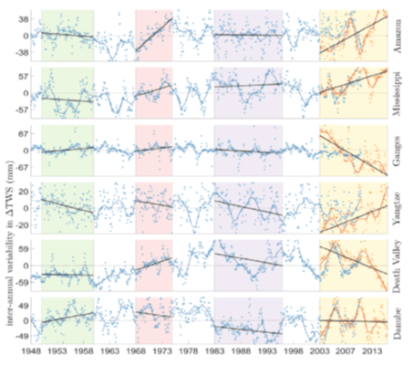
Figure 1. An illustration of how short-term trends in terrestrial water storage (ΔTWS) for six major river catchments – as highlighted by the coloured bars and comparable in length to those obtained from GRACE – are dependent on the time-period selected and do not always provide a reliable indicator of longer-term change. [Source: Vishwakarma et al. (2020) DOI: 10.1088/1748-9326/abd4a9]
To improve this, we introduce a new metric (Trend to Variability ratio, TVR) for assessing the severity of GRACE trends with regards past variability and show that GRACE-derived water storage trends are better interpreted when set in the context of historical variability. Using GRACE data complemented by TVR, we find that several regions thought to be losing water at a moderate rate are more endangered when longer term natural variability is considered, and vice-versa. We also estimate that greater than 3.2 billion people are currently living in regions facing severe water storage depletion, and that over one-third of river catchments that lost water in the last decade have suffered unprecedented losses.
(3) Attributing variability in coastal sea level short time series
Our BHM framework aims to solve the sea level budget and will initially use the `golden period’ of overlapping Argo and GRACE missions (2005 to 2015), with 11 years of excellent quality and high spatial resolution data. Sea level changes on inter-annual to decadal time scales are driven in-part by internal variability, particularly from climatic atmosphere-ocean interactions. To better understand what this internal variability can look like, we have also been asking: how much of the decadal, coastal sea level variability can be described by climate modes?
We have determined spatial patterns of sea level variability from a high-resolution ocean-model and compared decadal time series against key climate indices that describe large-scale climate variability. In doing so, we obtain reconstructed time series of the decadal sea level variability with a known source (e.g. Figure 2). Reducing the observed sea level by these reconstructions can reduce the uncertainty in trend and acceleration estimates and clarifies the signal from other sources in the sea level budget. We will be reporting more results from this work later in 2021.

Figure 2. The percentage of variance in sea level decadal time series that can be explained by a reconstructed time series using only climate indices (like the El Nino Southern Oscillation, or ENSO, index). Whilst the spatial picture is complex there are regions, including those that are observation-poor like the West African coast, where we can account for much sea level variability from simple indices. [Source: the authors]
New publications
Vishwakarma B.D., Bates, P., Sneeuw, N., Westaway, R.M. and Bamber, J. L. (2020). Re-assessing global water storage trends from GRACE time series. Environmental Research Letters (DOI:10.1088/1748-9326/abd4a9 ![]() ).
).
Vishwakarma, B. D., Royston, S., Riva, R. E. M., Westaway, R. M., & Bamber, J. L. (2020). Sea level budgets should account for ocean bottom deformation. Geophysical Research Letters 47, e2019GL086492 (DOI:10.1029/2019GL086492 ![]() ).
).
Royston, S., Vishwakarma, B. D., Westaway, R. M., Rougier, J., Sha, Z., and Bamber, J. L. (2020). Can we resolve the basin‐scale sea level trend budget from GRACE ocean mass? Journal of Geophysical Research: Oceans 125, e2019JC015535 (DOI:10.1029/2019JC015535).